Chapter 6 Two-Factor Designs with 1 Replicate per Treatment
In some cases, there is only a single replicate within each combination of factor levels. This causes a problem when considering models with interaction effects. The error degrees of freedom are \(df_E=ab(n-1)=ab(1-1)=0\) and the error sum of squares is \(SSE=0\). Several methods have been developed for testing for interaction under particular restrictions. In this chapter, we describe Tukey’s One Degree of Freedom for Non-Additivity Test (ODOFNA). For this test, the form of the interaction and the resulting test are given below.
\[ \left(\alpha\beta\right)_{ij} = D\alpha_i\beta_j \qquad \qquad H_0:D=0 \quad H_A:D\ne 0 \]
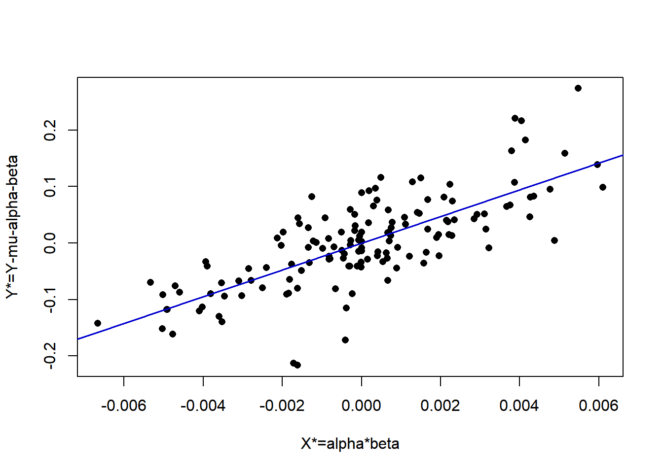
Intuitively, the test involves estimating \(\mu\), as well as \(\alpha_i\) and \(\beta_j\) from the marginal means for factors A and B. Then \(D\) is estimated by fitting a regression through the origin relating \(Y^*\) (\(Y\) minus the sum of the mean and the main effects) to \(X^*\) where \(X^*\) is the product of the estimates of \(\alpha_i\), and \(\beta_j\).
\[ \hat{\mu}=\overline{Y}_{\bullet\bullet}\qquad \hat{\alpha}_i = \overline{Y}_{i\bullet} - \overline{Y}_{\bullet\bullet}\qquad \hat{\beta}_j = \overline{Y}_{\bullet j} - \overline{Y}_{\bullet\bullet} \qquad Y_{ij}^*=Y_{ij}-\hat{\mu}-\hat{\alpha}_i-\hat{\beta}_j \qquad X_{ij}^*=\hat{\alpha}_i\hat{\beta}_j \]
For regression through the origin, we obtain the estimate and test whether \(D=0\) as follows, where the model with \(D\) is the complete model.
\[ \hat{D}=\frac{\sum_{i=1}^a\sum_{j=1}^bX_{ij}^*Y_{ij}^*}{\sum_{i=1}^a\sum_{j=1}^bX_{ij}^{*2}} \qquad \hat{Y}_{ij}(C)=\hat{\mu}_{\bullet\bullet}+\hat{\alpha}_i + \hat{\beta}_j + \hat{D}\hat{\alpha}_i\hat{\beta}_j \qquad i=1,\ldots,a; \quad j=1,\ldots,b \] \[ SSE(C)=\sum_{i=1}^a\sum_{j=1}^b\left(Y_{ij}-\hat{Y}_{ij}(C)\right)^2 \qquad df_E(C)=ab-(a-1)-(b-1)-1=ab-a-b+1 \] Under the reduced model, \(D=0\), and we obtain the following fitted values and error sum of squares and degrees of freedom.
\[ \hat{Y}_{ij}(R)=\hat{\mu} + \hat{\alpha}_i + \hat{\beta}_j \qquad SSE(R)=\sum_{i=1}^a\sum_{j=1}^b\left(Y_{ij}-\hat{Y}_{ij}(R)\right)^2 \qquad df_E(R)=ab-a-b+2 \]
Then Tukey’s ODOFNA test is a special case of the general linear test with \(H_0:D=0\) vs \(H_A:D \ne 0\).
\[ \mbox{Test Statistic:} \quad F^*=\frac{\left[\frac{SSE(R)-SSE(C)}{df_E{R}-df_E(C)}\right]} {\left[\frac{SSE(C)}{df_E(C)}\right]} \qquad \mbox{Rejection Region:} \quad F^*\ge F_{1-\alpha;1,ab-a-b} \]
6.1 Example - Economic Indices for 8 Sources Over 18 Years
A study considered U.S. economic indices for \(a=8\) business news sources over a \(b=18\) year period (Smith 1969). The sources were: DJIA, Poors, NYSE, GNP, CPI, Forbes, Business Week, and Money Magazine. The years were 1948-1965. There was one index per source per year. The following R code runs calculations directly, then structures the data in matrix form and uses the additivityTests package. Note that we order the data frame first by source, then by year within source, as tapply output is sorted by the alphanumeric levels of the grouping variable(s).
biz1 <- read.table("http://www.stat.ufl.edu/~winner/data/jb42.dat",header=F,
    col.names=c("source","year","Y"))
head(biz1)
## source year Y
## 1 DJIA 1965 1.103
## 2 DJIA 1964 1.145
## 3 DJIA 1963 1.169
## 4 DJIA 1962 0.890
## 5 DJIA 1961 1.207
## 6 DJIA 1960 0.896## Create a new data frame that orders first by source then year within source
biz <- biz1[order(biz1$source, biz1$year),]
head(biz)## source year Y
## 126 BWEEK 1948 1.019
## 125 BWEEK 1949 0.995
## 124 BWEEK 1950 1.213
## 123 BWEEK 1951 1.012
## 122 BWEEK 1952 1.141
## 121 BWEEK 1953 0.952tail(biz)## source year Y
## 24 POOR 1960 0.953
## 23 POOR 1961 1.231
## 22 POOR 1962 0.872
## 21 POOR 1963 1.201
## 20 POOR 1964 1.131
## 19 POOR 1965 1.099all.mean <- mean(biz$Y)
source.mean <- as.vector(tapply(biz$Y, biz$source, mean))
year.mean <- as.vector(tapply(biz$Y, biz$year, mean))
a <- length(source.mean)
b <- length(year.mean)
biz$mu <- rep(all.mean, a*b)
biz$alpha <- rep(source.mean-all.mean, each=b)
biz$beta <- rep(year.mean-all.mean, times=a)
biz$Ystar <- biz$Y - biz$mu - biz$alpha - biz$beta
biz$Xstar <- biz$alpha * biz$beta
(Dhat <- sum(biz$Xstar*biz$Ystar) / sum(biz$Xstar^2))## [1] 23.6517biz$Yhat.C <- biz$mu + biz$alpha + biz$beta + Dhat*biz$Xstar
biz$Yhat.R <- biz$mu + biz$alpha + biz$beta
SSE.C <- sum((biz$Y-biz$Yhat.C)^2)
SSE.R <- sum((biz$Y-biz$Yhat.R)^2)
df_E.C <- a*b - a - b
df_E.R <- a*b - a - b + 1
Fstar <- ((SSE.R-SSE.C)/(df_E.R-df_E.C)) / (SSE.C/df_E.C)
odofna.out <- cbind(df_E.R, df_E.C, SSE.R, SSE.C, Fstar, qf(.95,1,df_E.C),
1-pf(Fstar,1,df_E.C))
colnames(odofna.out) <- c("df(R)", "df(C)", "SSE(R)", "SSE(C)", "F*", "F(.95)", "P(>F*)")
rownames(odofna.out) <- c("ODOFNA")
round(odofna.out, 4)## df(R) df(C) SSE(R) SSE(C) F* F(.95) P(>F*)
## ODOFNA 119 118 0.9305 0.4075 151.4522 3.9215 0plot(biz$Ystar ~ biz$Xstar, pch=16, xlab="X*=alpha*beta", ylab="Y*=Y-mu-alpha-beta")
abline(lm(Ystar ~ Xstar - 1,data=biz), col="blue3", lwd=1.5)
### biz is sorted by index, then year (stacked COLUMNS from spreadsheet)
(Y.mat <- matrix(biz$Y,byrow=F,ncol=8))
## [,1] [,2] [,3] [,4] [,5] [,6] [,7] [,8]
## [1,] 1.019 1.077 0.972 1.041 1.110 0.985 0.972 0.996
## [2,] 0.995 0.990 1.114 0.945 0.996 0.994 1.102 1.091
## [3,] 1.213 1.009 1.179 1.157 1.102 1.057 1.211 1.247
## [4,] 1.012 1.080 1.174 1.085 1.156 1.055 1.132 1.178
## [5,] 1.141 1.022 1.074 1.037 1.055 1.038 1.065 1.109
## [6,] 0.952 1.008 0.965 1.083 1.053 1.010 0.938 0.925
## [7,] 1.074 1.004 1.393 0.940 0.994 1.029 1.426 1.497
## [8,] 1.125 0.997 1.231 1.126 1.095 1.020 1.222 1.301
## [9,] 1.011 1.015 1.000 1.034 1.055 1.012 1.026 1.034
## [10,] 0.906 1.035 0.833 1.008 1.056 0.993 0.866 0.856
## [11,] 1.099 1.028 1.425 0.930 1.044 1.038 1.366 1.376
## [12,] 1.073 1.008 1.184 1.127 1.086 1.006 1.097 1.094
## [13,] 0.917 1.016 0.896 1.029 1.041 0.924 0.976 0.953
## [14,] 1.154 1.011 1.207 1.099 1.032 1.031 1.240 1.231
## [15,] 1.018 1.012 0.890 1.078 1.072 1.013 0.880 0.872
## [16,] 1.060 1.012 1.169 1.051 1.050 1.038 1.180 1.201
## [17,] 1.073 1.013 1.145 1.064 1.066 1.043 1.143 1.131
## [18,] 1.093 1.017 1.103 1.083 1.086 1.048 1.095 1.099tukey.test(Y.mat)##
## Tukey test on 5% alpha-level:
##
## Test statistic: 151.5
## Critival value: 3.921
## The additivity hypothesis was rejected.There is strong evidence of an interaction between source and year, of this form.
\[ (\alpha\beta)_{ij} = D\alpha_i\beta_j \quad \mbox{ with } \hat{D}=23.65 \]
\[ \nabla \]